Display your results

Scientists love to present their results graphically, because like a picture is worth a thousand words, a good plot can replace a lot of tables. The python scene is full of libraries for data visualization, from the most basic like matplotlib offering a low level interface to higher level tools like seaborn where the user can profit from predefined classes to display complex relationships among different variables in the dataset.

In a spirit of complete freedom, MAFw is not deciding for you what plotting or data frame library you should use for your analysis. For this reason, we have prepared a skeleton of the generic plotter processor that you can use as a template and implement it with your favorite libraries.

Nevertheless, if you are ok with the use of seaborn as a data visualization platform (using matplotlib under the hood for the low level plotting routines) and pandas and numpy for data handling, then MAFw can offer you a pre-cooked solution implemented in the SNSPlotter.

If you want to use SNSPlotter, then you need to install mafw including the seaborn optional feature, in this way:

c:\> pip install mafw[seaborn]

In the next section of this unit, we will assume that you are using the seaborn functionalities.

Add diagnostic information to your processors

Processors are responsible for performing simple analysis tasks; however, it is essential to verify and assess the accuracy of their output. We strongly recommend to include the generation of some diagnostic plots or storing some key results in a database table while implementing the process() method in order to verify the correct execution of the analysis task.

This aspect is totally in your hand and MAFw has little to offer; you will have to code your Processor so that it can create meaningful figures.

Warning

For this diagnostic output you can use the graphical library of your choice, but many of you will opt for matplotlib given its widespread use in the field. This library allows you to decide which backend to use from a long list of options including interactive and not interactive choices. If you let matplotlib decide, it will use one of the available backends according to a precedence list. In many cases, this will be TkAgg that is known to have issues when used in a non interactive way with frequently opening and closure of figure windows. Those issues will appear as randomly occurring RuntimeError involving TclAsync or main thread not in main loop. In such a case, the solution is to switch to a non-interactive backend that is normally absolutely ok because usually diagnostic output is simply saved on files and not directly displayed to you. The simplest non interactive backend is Agg and it is built-in in matplotlib so no need to install anything else.

You can force matplotlib to select a specific backend via the environment variable MPLBACKEND simply setting it to agg. This decision will affect all scripts (including mafw execution engine). If you want something that is specific for one or many processors of yours, you can add the following lines of code to your processor start method.

try:
    my_backend == 'agg'
    if plt.get_backend() != my_backend:
        plt.switch_backend(my_backend)
except ModuleNotFoundError:
    log.critical('%s is not a valid plt backend' % my_backend)
    raise

You can even have a processor whose only task is to turn on and off interactivity. The reason why this is not an option available in the base Processor class is that MAFw is graphics agnostic and unless you install the optional feature seaborn otherwise matplotlib is not automatically installed.

Generate high level graphs

Along with graphs aimed to verify that your processor was actually behaving as expected, you might have the need to have processors whose main task is indeed the generation of high level figures to be used for your publications or presentations starting from a data frame.

In this case, MAFw is providing you a powerful tool: the generic plotter processor.

The SNSPlotter is a member of the processor_library package and represents a specialized subclass of a Processor [1] with a predefined process() method.

When you are subclassing a Processor, you are normally required to implement some methods and the most important of all is clearly the process() one, where your analytical task is actually coded.

For a SNSPlotter, the process method is already implemented and it looks like the following code snipped:

def process(self) -> None:
    """
    Process method overload.

    In the case of a plotter subclass, the process method is already implemented and the user should not overload
    it. On the contrary, the user must overload the other implementation methods described in the general
    :class:`class description <.SNSPlotter>`.
    """
    if self.filter_register.new_only:
        if self.is_output_existing():
            return

    self.in_loop_customization()
    self.get_data_frame()
    self.patch_data_frame()
    self.slice_data_frame()
    self.group_and_aggregate_data_frame()
    if not self.is_data_frame_empty():
        self.plot()
        self.customize_plot()
        self.save()
        self.update_db()

In its basic form, all the methods included in the process have an empty implementation, and it is your task to make them doing something.

We can divide these methods into two blocks:

• The data handling methods: where the data frame is acquired and prepared for the plotting step.

  1. get_data_frame()

  2. patch_data_frame()

  3. slice_data_frame()

  4. group_and_aggregate_data_frame()

• The plotting methods: where you will have to generate the figures from the data frame and save them.

  1. plot()

  2. customize_plot()

  3. save()

  4. update_db()

Getting the data

The first thing to do when you want to plot some data is to have the data! The SNSPlotter has a data_frame attribute to store a pandas data frame exactly for this purpose. The data frame can be read in from a file or retrieved from a database table or even built directly in the processor itself. The get_data_frame() is the place where this is happening. It is important that you assign the data frame to self.data_frame attribute so that the following methods can operate on it.

The following three methods are giving you the possibility to add new columns based on the existing ones (patch_data_frame()), selecting a sub set of rows (slice_data_frame()) and grouping / aggregating the rows (group_and_aggregate_data_frame()).

Data frame patching

Use this method to add or modify data frame columns. One typical example is the application of unit of measurement conversion: you may want to store the data using the SI unit, but it is more convenient to display them using another more practical unit. Another interesting application is to replace numerical categorical values with textual one: for example you may want to add a column with the sample name to replace the column with the sample identification number. You can implement all these operations overloading the patch_data_frame() method. Below is an example of how to add an additional column that represents the exposure time of an image acquisition in hours, converted from the stored value in seconds.

self.data_frame['ExposureTimeH'] = self.data_frame['ExposureTime'] / 3600.

Slicing the data frame

Use this method to select a specific group of rows, corresponding to a certain value for a variable. You do not need to overload the slice_data_frame(), but just define the slicing_dict attribute and the basic implementation will do the magic. Have a look also at the documentation of the function slice_data_frame() from the pandas_tools module. In a few words, if you have a data frame with four columns named A, B, C and D and you want to select only the rows where column A is equal to 10, then set self.slicing_dict = { 'A' : 10 } and the slice_data_frame() method will do the job for you.

Group and aggregate the data frame

In a similar manner, you can group and aggregate the columns of the data frame by defining the grouping columns and aggregation functions attributes. Also for this method, have a look at the group_and_aggregate_data_frame() function from the pandas_tools. If, for example, you have a data frame containing two columns named SampleName and Signal and you want to get the average and standard deviation of the signal column for each of the different samples, then you can do:

self.grouping_columns = ['SampleName']
self.aggregation_functions = ['mean', 'std']

The group_and_aggregate_data_frame() will perform the grouping and aggregation and assign to the self.data_frame a modified data frame with three columns named SampleName, Signal_mean and Signal_std.

Per cycle customization

You may wonder, when and where in your code you should be setting the slicing and grouping / aggregating parameters. Those values can be ‘statically’ provided directly in the constructor of the generic plotter processor subclass, but you can also have them dynamically assigned at run time overloading the in_loop_customization() method.

In the implementation of this method you can also set other parameters relevant for your plotting.

Plotting the data

Now that you have retrieved and prepared your data frame, you can start the real plotting. First of all, just be sure that after all your modifications, the data frame is still containing some rows, otherwise, just move on to the next iteration.

The generation of the real plot is done in the implementation of the plot(). The SNSPlotter is meant to operate with seaborn so it is quite reasonable to anticipate that the results of the plotting will be assigned to a facet grid attribute, in order to allow the following methods to refer to the plotting output.

If your plot() implementation is not actually generating a facet grid, but something else, it is still ok. If you want to pass a static typing, then define a attribute in your SNSPlotter subclass with the proper typing; if you are not doing any static typing you can still use the facet grid attribute for storing your object.

Customising the plot

When producing high quality graphs, you want to have everything looking perfect. You can implement this method to set the figure and plot titles, the axis labels and to add specific annotations. If your SNSPlotter implementation is following a looping execution workflow, you can use the looping parameters if you need them. Theoretically speaking you could code this customisation directly in the plot method, but the reason for this split will become clear later on when explaining the mixin approach.

Save the plot

This is where your figure must be saved to a file. The very typical implementation of this method is the following:

def save(self) -> None:
    self.facet_grid.figure.savefig(self.output_filename)
    self.output_filename_list.append(self.output_filename)

This is assuming that your SNSPlotter subclass has an attribute (it can also be a processor parameter) named output_filename. The second statement is also very common: the SNSPlotter has a list type attribute to store the names of all generated files. This list, along with the cumulative checksum will be stored in the dedicated PlotterOutput standard table, to avoid the regeneration of identical plots. You do not have to worry about updating this standard table, this operation will be performed automatically by the private method _update_plotter_db().

Update the db

Along with the PlotterOutput standard table, you may want to update also other objects in the database. For this purpose, you can implement the update_db() method.

Mixin approach

You might have noticed that the structure of the process() is a bit over-granular. The reason behind this fine distinction is due to the fact that the code can potentially be reused to a large extent thanks to a clever use of mixin classes.

Explanation

If you are not a seasoned programmer, you might not be familiar with the concept of mixins. Those are small classes implementing a specific subtask of a bigger class, finding extensive usage in developing interfaces. If you wish, you can have a general explanation following this webpage.

If you are aware of what a mixin is and how to use it, then just go to the next section.

In the case of the SNSPlotter, we have seen that its methods can be divided into two categories: the data retriever and the actual plotter. You can have several different data retriever options and also different plotting strategies, thus making the creation of a matrix of subclasses of the SNSPlotter covering all possible cases really unpractical.

The mixin approach allows to have a flexible subclass scheme and at the same time an optimal reuse of code units.

To make things even more evident, here is a logical scheme of what happens when you mix a DataRetriever mixin with a SNSPlotter.

Let us start from the definition of the subclass itself:

class MyPlotterSNS(MyDataRetrieverMixin, MyPlotMixin, SNSPlotter):

MyPlotterSNS is mixing two mixins, one DataRetriever and one FigurePlotter, with the SNSPlotter. The order matters: always put mixins before the base class, because this is affecting the method resolution order (MRO) that follows a depth-first left-to-right traversal.

MyDataRetrieverMixin being a subclass of DataRetriever is implementing these two methods get_data_frame() and patch_data_frame() that are also defined in the SNSPlotter.

During the execution of the process(), the get_data_frame method will be called and, thanks to the MRO, the MyDataRetrieverMixin will provide its implementation of such method. The same will apply for the plot, where the MyPlotMixin will kick in and provide its implementation of the method.

Mixins can come with other class parameters along with the ones shared with the base class. Those can be accessed and assigned using the standard dot notation on the instances of the mixed class, or they can also be defined in the mixed class constructor directly.

Data-retriever mixins

Let us start considering the data retrieval part. Very likely, you will get those data either from a database table or from a HDF5 file. If this is the case, then you do not need to code the get_data_frame method everytime, but you can use one of the available mixin to grab the data.

For the moment, the following data retriever mixins exist [2]:

• HDFPdDataRetriever.

  This data retriever is opening the provided HDF5 file name and obtaining the data frame identified by the provided key.

• SQLPdDataRetriever.

  This data retriever is performing a SQL query on a table (table_name) using as columns the provided required_columns list and fulfilling the where_clause. A valid database connection must exist for this retriever to work, it means that the processor with which this class is mixed must have a working database instance.

• FromDatasetDataRetriever.

  This data retriever is provided mainly for test and debug purposes. It allows to obtain a data frame from the standard data set library of seaborn.

If you plan to retrieve data several times from a common source, you may consider to add your own mixin class. Just make it inheriting from the DataRetriever (or PdDataRetriever if you are using Pandas) class and follow one of the provided case as an example.

Here below is an example of a Plotter retrieving the data from a HDF file:

@single_loop
class HDFPlotterSNS(HDFDataRetriever, SNSPlotter):
    pass

hdf = HDFPlotterSNS(hdf_filename=your_input_file, key=your_key)
hdf.execute()

The hdf_filename and the key can be provided directly in the class constructor, but this might not doable if you are planning to execute the processor using the mafw steering file approach.

In this case, you can add two parameters to your processor that can be read from the steering file and follow this approach:

@single_loop
class HDFPlotterSNS(HDFDataRetriever, SNSPlotter):
    hdf_filename_from_steering = ActiveParameter('hdf_filename_from_steering', default='my_datafile.h5')
    hdf_key_from_steering = ActiveParameter('hdf_key_from_steering', default='my_key')

    def start(self):
        super().start()
        # you can assign the parameter values to the mixin attributes in the start method
        # but also in the in_loop_customization method if this is better suiting your needs
        self.hdf_filename = self.hdf_filename_from_steering
        self.key = self.hdf_key_from_steering

# let us execute the processor from within the mafw runner.

Figure plot mixins

In a similar way, if what you want is to generate a seaborn figure level plot, then you do not need to define the plot method every time. Just mix the SNSPlotter with one of the four figure plotter mixins available:

• RelPlot: to plot relational plots.

• DisPlot: to plot distribution graphs.

• CatPlot: to produce categorical figures.

• LMPlot: to produce linear regression model figures.

From the coding point of it, the approach is identical to the one shown before for the data retrieving mixin.

@single_loop
@processor_depends_on_optional(module_name='pandas;seaborn')
class DataSetRelPlotPlotterSNS(FromDatasetDataRetriever, RelPlot, SNSPlotter):
    def __init__(self, output_png: str | Path | None = None, *args: Any, **kwargs: Any) -> None:
        super().__init__(*args, **kwargs)
        self.output_png = Path(output_png) if output_png is not None else Path()

    def save(self) -> None:
        self.facet_grid.figure.savefig(self.output_png)
        self.output_filename_list.append(self.output_png)

output_file = tmp_path / Path('relplot_from_dataset.png')

dsrp = DataSetRelPlotPlotterSNS(
    output_file, dataset_name='penguins', x='flipper_length_mm', y='bill_length_mm', col='sex', hue='species'
)
dsrp.execute()

The code above will generate this plot:

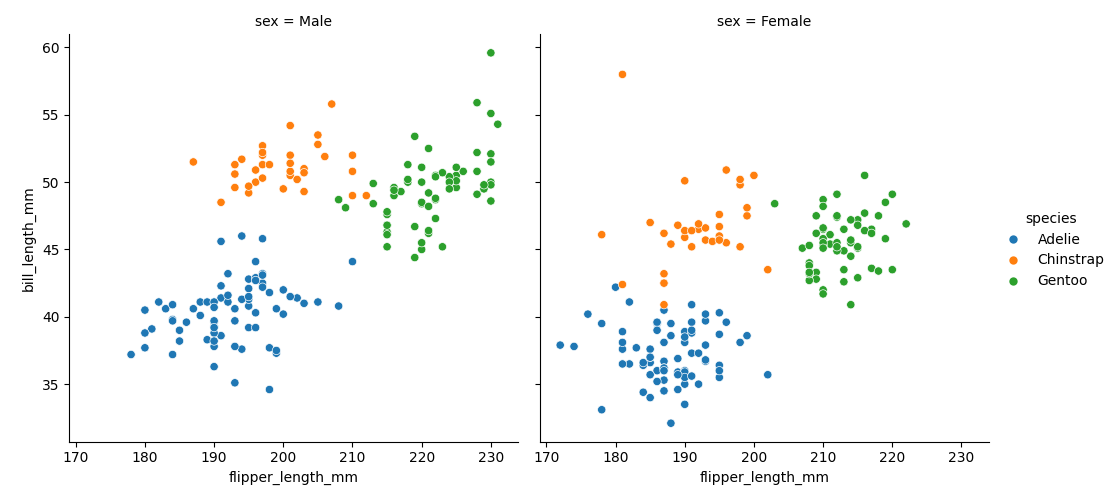
Fig. 8 This is the exemplary output of a SNSPlotter mixed with a data retriever and a relational plot mixin.

As you can see, the plot method is taken from the RelPlot mixin and the output can be further customized (axis labels and similar things) implementing the customize_plot method.

A large fraction of the parameters that can be passed to the seaborn figure level functions corresponds to attributes in the mixin class, but not all of them. For the missing ones, you can use the dictionary like parameter plot_kws, to have them passed to the underlying plotting function. See the documentation of the mixins for more details (RelPlot, DisPlot and CatPlot).

Footnotes

[1]

Actually SNSPlotter parent class is GenericPlotter that is a subclass of Processor. This intermediate inheritance step is needed to allow the user to define their preferred interface to graphical and data frame library.

[2]

The extra Pd in the name of these classes stands for Pandas. In fact the user is free to select any other data frame library and define their own data retriever mixin.