Note
Note for direct readers: If you have navigated directly to this practical example without reading the preceding documentation, please be aware that this implementation demonstrates advanced concepts and methodologies that are thoroughly explained in the earlier sections. While this example is designed to be self-contained, some technical details, and design decisions may not be immediately clear without the foundational knowledge provided in the main documentation. Should you encounter unfamiliar concepts or require deeper understanding of the library’s architecture and principles, we recommend referring back to the relevant sections of the complete documentation.
A step by step tutorial for a real experimental case study
Congratulations! You have decided to give a try to MAFw for your next analysis, you have read all the documentation provided, but you got overwhelmed by information and now you do not know from where to start.
Do not worry, we have a simple, but nevertheless complete example that will guide you through each and every steps of your analysis.
Before start typing code, let’s introduce the experimental scenario.
The experimental scenario
Let’s imagine, that we have a measurement setup integrating the amount of UV radiation reaching a sensor in a give amount of time.
The experimental data acquisition (DAQ) system is saving one file for each exposure containing the value read by the sensor. The DAQ is encoding the duration of the acquisition in the file name and let’s assume we acquired 25 different exposures, starting from 0 up to 24 hours. The experimental procedure is repeated for three different detectors having different type of response and the final goal of our experiment is to compare their performance.
It is an ultra simplified experimental case and you can easily make it as complex as you wish, just by adding other variables (different UV lamps, detector operating conditions, background illumination…). Nevertheless this simple scenario can be straightforward expanded to any real experimental campaign.
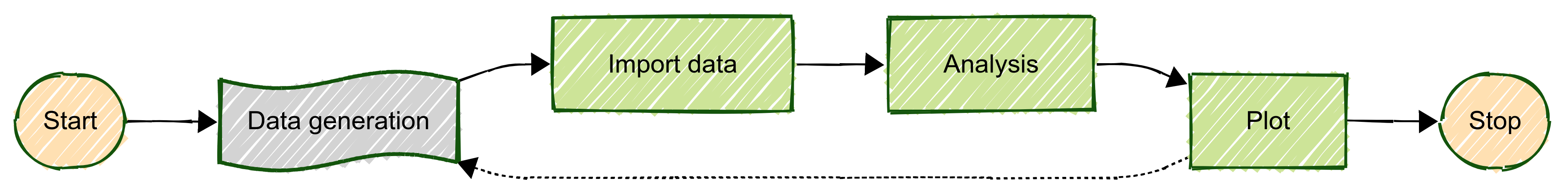
Fig. 10 The simplified pipeline for the tutorial example.
Task 0. Generating the data
This is not really an analysis task, rather the real acquisition of the data, that’s why it is represented with a
different color in schema above. Nevertheless it is important to include that in our planning, because new data might
be generated during or after some data have been already analyzed. In this case, it is important that our analysis
pipelines will be able to process only the new (or modified) data, without wasting time and resources re-doing what has
been done already. This is the reason why there is a dashed line looping back from the plot step to the data generation.
Since this is a simulated experiment, instead of collecting real data, we will use a Processor to generate
some synthetic data.
Task 1. Building your data bank
From a conceptual point of view, the first thing you should do when using MAFw is to import all your data (in this case the raw data files) into a relational database. You do not need to store the content of the file in the database, otherwise it will soon explode in size, you can simply insert the full path from where the file can be retrieved and its checksum, so that we can keep an eye on possible modifications.
Task 2. Do the analysis
In the specific scenario the analysis is very easy. Each file contains only one number, so there is very little to be done, but your case can be as complicated as needed. We will open each file, read the content and then put it in a second database table containing the results of the analysis of each file. In your real life experiment, this stage can contain several processors generating intermediate results stored as well in the database.
Task 3. Prepare a relation plot
Using the data stored in the database, we can generate a plot representing the integral flux versus the exposure time for the three different detectors using a relation plot.
The ‘code’
In the previous section, we have defined what we want to achieve with our analysis (it is always a good idea to have a plan before start coding!). Now we are ready to start with setting up the project containing the required processors to achieve the analytical goal described above.
If you want to use MAFw plugin mechanism, then you need to build your project as a proper python package. Let’s start
then with the project specification contained in the pyproject.toml file.
 1[build-system]
 2requires = ["hatchling"]
 3build-backend = "hatchling.build"
 4
 5[project]
 6name = "plug_test"
 7dynamic = ["version"]
 8description = 'A MAFw processor library plugin'
 9readme = "README.md"
10requires-python = ">=3.11"
11license = "EUPL-1.2"
12authors = [
13  { name = "Antonio Bulgheroni", email = "antonio.bulgheroni@ec.europa.eu" },
14]
15classifiers = [
16  "Development Status :: 4 - Beta",
17  "Programming Language :: Python",
18  "Programming Language :: Python :: 3.11",
19  "Programming Language :: Python :: 3.12",
20  "Programming Language :: Python :: 3.13",
21  "Programming Language :: Python :: Implementation :: CPython",
22  "Programming Language :: Python :: Implementation :: PyPy",
23]
24
25dependencies = ['mafw', 'pluggy']
26
27[project.urls]
28Documentation = "https://github.com/..."
29Issues = "https://github.com/..."
30Source = "https://github.com/."
31
32[project.entry-points.mafw]
33plug_test = 'plug.plugins'
34
35[tool.hatch.version]
36path = "src/plug/__about__.py"
37
38[tool.hatch.build.targets.wheel]
39packages = ['src/plug']
The specificity of this configuration file is in the highlighted lines: we define an entry point where your processors are made available to MAFw.
Now before start creating the rest of the project, prepare the directory structure according to the python packaging specification. Here below is the expected directory structure.
plug
├── README.md
├── pyproject.toml
└── src
    └── plug
        ├── __about__.py
        ├── db_model.py
        ├── plug_processor.py
        └── plugins.py
You can divide the code of your analysis in as many python modules as you wish, but for this simple project we will keep all processors in one single module plug_processor.py. We will use a second module for the definition of the database model classes (db_model.py). Additionally we will have to include a plugins.py module (this is the one declared in the pyproject.toml entry point definition) where we will list the processors to be exported along with our additional standard tables.
The database definition
Let’s move to the database definition.
Our database will contain tables corresponding to the three model classes: InputFile and Data, and one helper table for the detectors along with all the standard tables that are automatically created by MAFw.
Before analysing the code let’s visualize the database with the ERD.

Fig. 11 The schematic representation of our database. The standard tables, automatically created are in green. The detector table (yellow) is exported as a standard table and its content is automatically restored every time mafw is executed.
The InputFile is the model where we will be storing all the data files that are generated in our experiment while the Data model is where we will be storing the results of the analysis processor, in our specific case, the value contained in the input file.
The rows of these two models are linked by a 1-to-1 relation defined by the primary key.
Remember that is always a good idea to add a checksum field every time you have a filename field, so that we can check if the file has changed or not.
The InputFile model is also linked with the Detector model to be sure that only known detectors are added to the analysis.
Let’s have a look at the way we have defined the three models.
 1class Detector(StandardTable):
 2    detector_id = AutoField(primary_key=True, help_text='Primary key for the detector table')
 3    name = TextField(help_text='The name of the detector')
 4    description = TextField(help_text='A longer description for the detector')
 5
 6    @classmethod
 7    def init(cls) -> None:
 8        data = [
 9            dict(detector_id=1, name='Normal', description='Standard detector'),
10            dict(detector_id=2, name='HighGain', description='High gain detector'),
11            dict(detector_id=3, name='NoDark', description='Low dark current detector'),
12        ]
13
14        cls.insert_many(data).on_conflict(
15            conflict_target=[cls.detector_id],
16            update={'name': SQL('EXCLUDED.name'), 'description': SQL('EXCLUDED.description')},
17        ).execute()
The detector table is derived from the StandardTable, because we want the possibility to initialize the content of this table every time the application is executed. This is obtained in the init method. The use of the on_conflict clause assure that the three detectors are for sure present in the table with the value given in the data object. This means that if the user manually changes the name of one of these three detectors, the next time the application is executed, the original name will be restored.
 1class InputFile(MAFwBaseModel):
 2    @classmethod
 3    def triggers(cls) -> list[Trigger]:
 4        update_file_trigger = Trigger(
 5            trigger_name='input_file_after_update',
 6            trigger_type=(TriggerWhen.After, TriggerAction.Update),
 7            source_table=cls,
 8            safe=True,
 9            for_each_row=True,
10        )
11        update_file_trigger.add_when(or_('NEW.exposure != OLD.exposure', 'NEW.checksum != OLD.checksum'))
12        update_file_trigger.add_sql('DELETE FROM data WHERE file_pk = OLD.file_pk;')
13
14        return [update_file_trigger]
15
16    file_pk = AutoField(primary_key=True, help_text='Primary key for the input file table')
17    filename = FileNameField(unique=True, checksum_field='checksum', help_text='The filename of the element')
18    checksum = FileChecksumField(help_text='The checksum of the element file')
19    exposure = FloatField(help_text='The duration of the exposure in h')
20    detector = ForeignKeyField(
21        Detector, Detector.detector_id, on_delete='CASCADE', backref='detector', column_name='detector_id'
22    )
The InputFile has five columns, one of which is a foreign key linking it to the Detector model. Note that we have used
the FileNameField and FileChecksumField to take advantage of the verify_checksum() function. InputFile has a
trigger that is executed after each update that is changing either the exposure or the file content (checksum). When
one of these conditions is verified, then the corresponding row in the Data file will be removed, because we want to
force the reprocessing of this file since it has changed.
A similar trigger on delete is actually not needed because the Data model is linked to this model with an on_delete
cascade option.
 1class Data(MAFwBaseModel):
 2    @classmethod
 3    def triggers(cls) -> list[Trigger]:
 4        delete_plotter_sql = 'DELETE FROM plotter_output WHERE plotter_name = "PlugPlotter";'
 5
 6        insert_data_trigger = Trigger(
 7            trigger_name='data_after_insert',
 8            trigger_type=(TriggerWhen.After, TriggerAction.Insert),
 9            source_table=cls,
10            safe=True,
11            for_each_row=False,
12        )
13        insert_data_trigger.add_sql(delete_plotter_sql)
14
15        update_data_trigger = Trigger(
16            trigger_name='data_after_update',
17            trigger_type=(TriggerWhen.After, TriggerAction.Update),
18            source_table=cls,
19            safe=True,
20            for_each_row=False,
21        )
22        update_data_trigger.add_when('NEW.value != OLD.value')
23        update_data_trigger.add_sql(delete_plotter_sql)
24
25        delete_data_trigger = Trigger(
26            trigger_name='data_after_delete',
27            trigger_type=(TriggerWhen.After, TriggerAction.Delete),
28            source_table=cls,
29            safe=True,
30            for_each_row=False,
31        )
32        delete_data_trigger.add_sql(delete_plotter_sql)
33
34        return [insert_data_trigger, delete_data_trigger, update_data_trigger]
35
36    file_pk = ForeignKeyField(InputFile, on_delete='cascade', backref='file', primary_key=True, column_name='file_id')
37    value = FloatField(help_text='The result of the measurement')
The Data model has only two columns, one foreign key linking to the InputFile and one with the value calculated by the Analysis processor. It is featuring three triggers executed on INSERT, UPDATE and DELETE. In all these cases, we want to be sure that the output of the PlugPlotter is removed so that a new one is generated. Keep in mind that when a row is removed from the PlotterOutput model, the corresponding files are automatically added to the OrphanFile model for removal from the filesystem the next time a processor is executed.
Via the use of the foreign key, it is possible to associate a detector and the exposure for this specific value.
The processor library
Let’s now prepare one processor for each of the tasks that we have identified in our planning. We will create a processor also for the data generation.
GenerateDataFiles
This processor will accomplish Task 0 and it is very simple. It will generate a given number of files containing one single number calculated given the exposure, the slope and the intercept. The detector parameter is used to differentiate the output file name. As you see here below, the code is very simple.
 1class GenerateDataFiles(Processor):
 2    n_files = ActiveParameter('n_files', default=25, help_doc='The number of 1-h increasing exposure')
 3    output_path = ActiveParameter(
 4        'output_path', default=Path.cwd(), help_doc='The path where the data files are stored.'
 5    )
 6    slope = ActiveParameter(
 7        'slope', default=1.0, help_doc='The multiplication constant for the data stored in the files.'
 8    )
 9    intercept = ActiveParameter(
10        'intercept', default=5.0, help_doc='The additive constant for the data stored in the files.'
11    )
12    detector = ActiveParameter(
13        'detector', default=1, help_doc='The detector id being used. See the detector table for more info.'
14    )
15
16    def __init__(self, *args, **kwargs):
17        super().__init__(*args, **kwargs)
18        self.n_digits = len(str(self.n_files))
19
20    def start(self) -> None:
21        super().start()
22        self.output_path.mkdir(parents=True, exist_ok=True)
23
24    def get_items(self) -> Collection[Any]:
25        return list(range(self.n_files))
26
27    def process(self) -> None:
28        current_filename = self.output_path / f'rawfile_exp{self.i_item:0{self.n_digits}}_det{self.detector}.dat'
29        value = self.i_item * self.slope + self.intercept
30        with open(current_filename, 'wt') as f:
31            f.write(str(value))
32
33    def format_progress_message(self) -> None:
34        self.progress_message = f'Generating exposure {self.i_item} for detector {self.detector}'
In order to generate the different detectors, you run the same processor with different values for the parameters.
PlugImporter
This processor will accomplish Task 1, i.e. import the raw data file into our database. This processor is inheriting
from the basic Importer so that we can use the functionalities of the FilenameParser.
 1@database_required
 2class PlugImporter(Importer):
 3    def __init__(self, *args: Any, **kwargs: Any) -> None:
 4        super().__init__(*args, **kwargs)
 5        self._data_list: list[dict[str, Any]] = []
 6
 7    def get_items(self) -> Collection[Any]:
 8        pattern = '**/*dat' if self.recursive else '*dat'
 9        input_folder_path = Path(self.input_folder)
10
11        file_list = [file for file in input_folder_path.glob(pattern) if file.is_file()]
12
13        # verify the checksum of the elements in the input table. if they are not up to date, then remove the row.
14        verify_checksum(InputFile)
15
16        if self.filter_register.new_only:
17            # get the filenames that are already present in the input table
18            existing_rows = InputFile.select(InputFile.filename).namedtuples()
19            # create a set with the filenames
20            existing_files = {row.filename for row in existing_rows}
21            # filter out the file list from filenames that are already in the database.
22            file_list = [file for file in file_list if file not in existing_files]
23
24        return file_list
25
26    def process(self) -> None:
27        try:
28            new_file = {}
29            self._filename_parser.interpret(self.item.name)
30            new_file['filename'] = self.item
31            new_file['checksum'] = self.item
32            new_file['exposure'] = self._filename_parser.get_element_value('exposure')
33            new_file['detector'] = self._filename_parser.get_element_value('detector')
34            self._data_list.append(new_file)
35        except ParsingError:
36            log.critical('Problem parsing %s' % self.item.name)
37            self.looping_status = LoopingStatus.Skip
38
39    def finish(self) -> None:
40        InputFile.insert_many(self._data_list).on_conflict_replace(replace=True).execute()
41        super().finish()
The get_items is using the verify_checksum() to verify that the table is still actual and we apply the filter
to be sure to process only new or modified files. The process and finish are very standard. In this specific case,
we preferred to add all the relevant information in a list and insert them all in one single call to the database.
But also the opposite approach (no storing, multiple insert) is possible.
Analyser
This processor will accomplish Task 2, i.e. the analysis of the files. In our case, we just need to open the file, read the value and put it in the database.
 1@database_required
 2class Analyser(Processor):
 3    def get_items(self) -> Collection[Any]:
 4        self.filter_register.bind_all([InputFile])
 5
 6        if self.filter_register.new_only:
 7            existing_entries = Data.select(Data.file_pk).execute()
 8            existing = ~InputFile.file_pk.in_([i.file_pk for i in existing_entries])
 9        else:
10            existing = True
11
12        query = InputFile.join_dependent_models().where(self.filter_register.filter_all()).where(existing)
13
14        return query
15
16    def process(self) -> None:
17        with open(self.item.filename, 'rt') as fp:
18            value = float(fp.read())
19
20        Data.create(file_pk=self.item.file_pk, value=value)
21
22    def format_progress_message(self) -> None:
23        self.progress_message = f'Analysing {self.item.filename.name}'
Also in this case, the generation of the item list is done keeping in mind the possible filters the user is applying in the steering file. In this respect the use of the join_dependent_models() is very practical because it automatically generates a select joining all tables for which a foreign key relationship with the input one (InputFile in this case) exists. You do not have to worry to write the various multiple joins, MAFw will take care of doing it for you.
In the process, we are inserting the data directly to the database, so we will have one query for each item.
PlugPlotter
This processor will accomplish the last task, i.e. the generation of a relation plot where the performance of the three detectors is compared.
 1@database_required
 2@processor_depends_on_optional(module_name='seaborn')
 3@single_loop
 4class PlugPlotter(SQLPdDataRetriever, RelPlot, SNSPlotter):
 5    new_defaults = {
 6        'output_folder': Path.cwd(),
 7    }
 8
 9    def __init__(self, *args, **kwargs):
10        super().__init__(
11            *args,
12            table_name='data_view',
13            required_cols=['exposure', 'value', 'detector_name'],
14            x='exposure',
15            y='value',
16            hue='detector_name',
17            facet_kws=dict(legend_out=False, despine=False),
18            **kwargs,
19        )
20
21    def start(self) -> None:
22        super().start()
23
24        sql = """
25        CREATE TEMP VIEW IF NOT EXISTS data_view AS
26        SELECT
27            file_id, detector.detector_id, detector.name as detector_name, exposure, value
28        FROM
29            data
30            JOIN input_file ON data.file_id = input_file.file_pk
31            JOIN detector USING (detector_id)
32        ORDER BY
33            detector.detector_id ASC,
34            input_file.exposure ASC
35            ;
36        """
37        self.database.execute_sql(sql)
38
39    def customize_plot(self):
40        self.facet_grid.set_axis_labels('Exposure', 'Value')
41        self.facet_grid.figure.subplots_adjust(top=0.9)
42        self.facet_grid.figure.suptitle('Data analysis results')
43        self.facet_grid._legend.set_title('Detector type')
44
45    def save(self) -> None:
46        output_plot_path = self.output_folder / 'output.png'
47
48        self.facet_grid.figure.savefig(output_plot_path)
49        self.output_filename_list.append(output_plot_path)
This processor is a mixture of SQLPdDataRetriever, RelPlot and SNSPlotter. The SNSPlotter has already some parameters and with the new_defaults dictionary we over ride value of the output_folder to point to the current folder.
Looking at the init method, you might notice a strange thing, the table_name variable is set to data_view, that does not corresponding to any of our tables. The reason for this strangeness is quickly explained.
The SQLPdDataRetriever is generating a pandas Dataframe from a SQL query. In our database the data table contains only two columns: the file reference and the measured value, so we have no direct access to the exposure nor to the detector. To get these other fields we need to join the data table with the input_file and the detector ones. The solution for this problem is the creation of a temporary view containing this join query. Have a look at the start method. This view will be deleted as soon as the connection will be closed.
The plugin module
Everything is ready, we just have to make MAFw aware of our processors and our standard tables. We are missing just a few lines of code in the plugins module
 1import mafw
 2from mafw.lazy_import import LazyImportProcessor, ProcessorClassProtocol
 3
 4
 5@mafw.mafw_hookimpl
 6def register_processors() -> list[ProcessorClassProtocol]:
 7    return [
 8        LazyImportProcessor('plug.plug_processor', 'GenerateDataFiles'),
 9        LazyImportProcessor('plug.plug_processor', 'PlugImporter'),
10        LazyImportProcessor('plug.plug_processor', 'Analyser'),
11        LazyImportProcessor('plug.plug_processor', 'PlugPlotter'),
12    ]
13
14
15@mafw.mafw_hookimpl
16def register_db_model_modules() -> list[str]:
17    return ['plug.db_model']
The code is self-explaining. We need to invoke the processor hooks and return the list of processors. Instead of passing the real processor, we will use the processors proxies, so that we can defer the import of the processor modules when and if needed.
Run the code!
We are done with coding and we are ready to run our analysis.
First thing, we need to install our package in a separated python environment.
c:\> python -m venv my_venv
c:\> cd my_venv
c:\my_venv> bin\activate
(my_venv) c:\my_venv> pip install -e c:\path\to\plug
$ python -m venv my_venv
$ source my_venv/bin/activate
(my_venv) $ pip install -e /path/to/plug
Now verify that the installation was successful. If you run mafw list command you should get the list of all available processors including the three that you have created.
(my_venv) c:\my_venv> mafw list
(my_venv) $ mafw list
One last step, before running the analysis. We need to make the two steering files, one for the generation of the synthetic data and one for the real analysis and also the configuration file for the importer.
 1# file: generate-file.toml
 2processors_to_run = ["GenerateDataFiles#1", "GenerateDataFiles#2", "GenerateDataFiles#3"]
 3
 4# customise the name of the analysis
 5analysis_name = "integration-test-p1"
 6analysis_description = """Generating data files"""
 7available_processors = ["GenerateDataFiles"]
 8
 9[GenerateDataFiles]
10n_files = 25 # The number of files being generated.
11output_path = "/tmp/full-int/data" # The path where the data files are stored.
12slope = 1.0 # The multiplication constant for the data stored in the files.
13detector = 1 # The detector id being used. See the detector table for more info.
14
15["GenerateDataFiles#1"]
16intercept = 5.0 # The additive constant for the data stored in the files.
17slope = 1.0 # The multiplication constant for the data stored in the files.
18detector = 1 # The detector id being used. See the detector table for more info.
19
20["GenerateDataFiles#2"]
21intercept = 15.0 # The additive constant for the data stored in the files.
22slope = 5.0 # The multiplication constant for the data stored in the files.
23detector = 2 # The detector id being used. See the detector table for more info.
24
25["GenerateDataFiles#3"]
26intercept = 0.1 # The additive constant for the data stored in the files.
27slope = 0.2 # The multiplication constant for the data stored in the files.
28detector = 3 # The detector id being used. See the detector table for more info.
29
30[UserInterface] # Specify UI options
31interface = "rich" # Default "rich", backup "console"
# file: analysis.toml
processors_to_run = ["TableCreator","PlugImporter","Analyser", "PlugPlotter"]

# customise the name of the analysis
analysis_name = "integration-test-p2"
analysis_description = """Analysing data"""
available_processors = ["PlugImporter", "Analyser", "PlugPlotter"]
new_only = true

[DBConfiguration]
URL = "sqlite:////tmp/full-int/plug.db" # Change the protocol depending on the DB type. Update this file to the path of your DB.

[DBConfiguration.parameters.sqlite]

[DBConfiguration.parameters.sqlite.pragmas] # Leave these default values, unless you know what you are doing!
journal_mode = "wal"
cache_size = -64000
foreign_keys = 1
synchronous = 0

[TableCreator] # Processor to create all tables in the database.
apply_only_to_prefix = [] # Create only tables whose name start with the provided prefixes.
force_recreate = false

[PlugImporter]
input_folder = "/tmp/full-int/raw_data" # The input folder from where the images have to be imported.
parser_configuration = "/tmp/full-int/importer_config.toml" # The path to the TOML file with the filename parser configuration
recursive = true

[Analyser]

[PlugPlotter]
output_plot_path = "/tmp/full-int/output.png" # The filename of the output plot

[UserInterface] # Specify UI options
interface = "rich" # Default "rich", backup "console"
 1# file: importer_config.toml
 2elements = ['exposure', 'detector']
 3
 4[exposure]
 5regexp = '[_-]*exp(?P<exposure>\d+\.*\d*)[_-]*'
 6type='float'
 7
 8[detector]
 9regexp = '[_-]*det(?P<detector>\d+)[_-]*'
10type='int'
Adapt the steering files, in particular the paths and you are ready to run! In the analysis TOML file, you will also find the section concerning the database; for this simple case we used a SQLite single file DB, but whatever other DB would work exactly in the same way.
(my_venv) c:\my_venv> mafw run generate-file.toml
(my_venv) $ mafw run generate-file.toml
This will run the GenerateDataFiles processor three times, as specified in the three replicas, one for each detector. In the steering file, you can see that there are base settings specified in the base GenerateDataFiles table, plus some specific values for the three replicas. If you need are refresh on processor replicas, go back here. The three processor replicas will generate all our input data and we are ready to start the data analysis.
(my_venv) c:\my_venv> mafw run analysis.toml
(my_venv) $ mafw run analysis.toml
And here comes the magic! The three processors will be executed one after the other, the database is created and filled with all the provided data and the comparison plot is generated (default file name output.png).
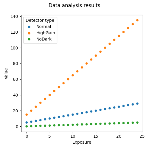
Fig. 12 The comparison plot of the three detectors.
This is just the beginning, now you can try all the benefits to use a clever database to drive your analysis pipeline. Try, for example, to remove one file and re-run the analysis, you will see a warning message informing you that a file was not found and that the corresponding row in the database has been removed as well. The rest of the analysis will remain the same, but the output plot will be regenerated with a missing point.
Try to manually modify the content of a file and re-run the analysis. The verify_checksum() will immediately
detect the change and force the re-analysis of that file and the generation of the output plot.
Try to rename one file changing the exposure value. You will see that mafw will detect that one file is gone missing in action, but a new one has been found. The output file will be update.
Try to repeat the analysis without any change and mafw won’t do anything! Try to delete the output plot and during the next run mafw will regenerate it.
You can also play with the database. Open it in DBeaver (be sure that the foreign_check is enforced) and remove one line from the input_file table. Run the analysis and you will see that the output plot file is immediately removed because it is no more actual and a new one is generated at the end of chain.
It’s not magic even if it really looks like so, it’s just a powerful library for scientists written by scientists!